The Data Infrastructure Behind Algorithmic Trading: Understanding Financial Data APIs

Algorithmic trading systems are often discussed in terms of models, signals, and execution logic. However, before any of these components can be developed, researchers must first solve a more fundamental problem: reliable access to financial data.

In professional research environments, data infrastructure is not a preliminary step. It is a gating function. If the data layer is inconsistent, every downstream model inherits that instability. In this article, we focus on the foundational layer of systematic trading: financial data infrastructure. We will explore how financial data APIs like FMP enable automated data ingestion, how they fit into quantitative research pipelines, and how developers can use them to build scalable research workflows using Python.

Why Data Infrastructure Matters in Algorithmic Trading

Data infrastructure determines whether a quantitative workflow can operate reliably at scale. Before models can be evaluated or signals can be tested, researchers must ensure that financial data is available in a structured, consistent, and scalable form. Without this foundation, even well-designed strategies become difficult to validate or reproduce.

Systematic Trading Requires Reliable Data Inputs

In systematic trading, data issues are rarely obvious at first. Small inconsistencies in inputs, such as missing values, misaligned timestamps, or formatting differences, propagate through the pipeline and distort feature calculations, model outputs, and backtest results.

Data Requirements in Quantitative Research

Quantitative workflows rely on multiple datasets that must integrate seamlessly, including price data, financial statements, and event-driven information. As research expands across larger universes and time periods, managing these datasets becomes increasingly complex without proper infrastructure.

Challenges with Manual Data Collection

In the absence of automation, data collection quickly becomes inefficient.

Manual workflows, such as downloading spreadsheets or copying data from multiple sources, introduce several limitations. These methods may work for small analyses, but do not scale well in a research environment.

Some common issues include:

• Differences in data formatting across sources
• Difficulty in maintaining updated datasets
• Limited scalability when working with many securities
• Reduced reproducibility of results

These challenges often lead to inconsistencies, making it difficult to validate research outcomes over time.

Financial Data APIs as the Foundation

Financial data APIs enable a structured and automated way to retrieve datasets directly into a research environment, replacing manual workflows with programmatic access.

In quantitative research pipelines, APIs primarily power the data ingestion layer, where datasets such as prices, financial statements, and estimates are retrieved and integrated directly into the workflow. This enables repeatable data access, easier integration with Python-based pipelines, and more scalable research processes.

What Is a Financial Data API

A financial data API enables programmatic access to financial datasets, allowing data to be retrieved directly within code rather than collected manually. It acts as an interface between a data provider and a research environment, enabling data to be requested and consumed directly inside code. In practice, developers also evaluate APIs based on latency, rate limits, schema consistency, and how reliably endpoints behave across large-scale requests.

In quantitative workflows, this means a Python script or notebook can retrieve datasets such as historical prices, financial statements, or analyst estimates without relying on manual downloads.

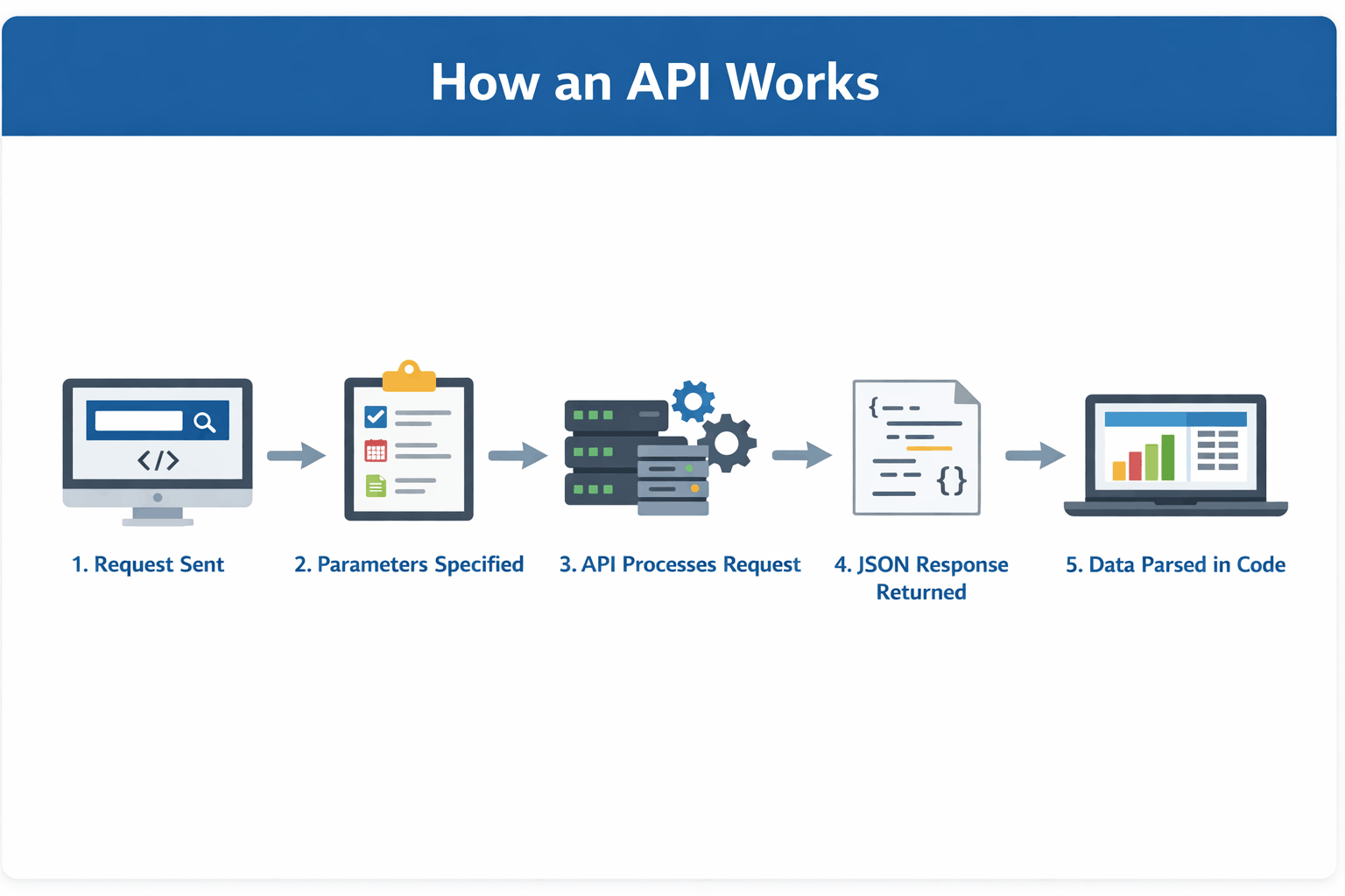
How an API Works in Practice

The following diagram summarises how a typical API interaction flows from request to data usage:

For example, financial data platforms expose endpoints for datasets such as company profiles, historical price data, and financial statements, all of which follow this request–response pattern.

Manual vs Programmatic Data Retrieval

The difference between manual workflows and API-based workflows becomes clear when comparing how data is collected

Aspect Manual Data Retrieval Programmatic Data Retrieval Effort High (repeated manual steps) Low (automated through code) Scalability Limited to small datasets Scales across large datasets Consistency Prone to formatting inconsistencies Standardised and structured Update Process Requires manual updates Automatically refreshable Reproducibility Difficult to replicate Fully reproducible workflows

For quantitative research, programmatic access is significantly more reliable because it reduces human intervention and ensures consistency.

Authentication Using API Keys

Most financial data APIs require authentication through an API key, which is included with each request. It verifies user identity and enables providers to manage access and usage limits.

Why APIs Are Central to Quant Workflows

Financial data APIs transform data access into a programmable component of the research pipeline. Instead of manual preparation, data retrieval becomes integrated directly into code, enabling consistent inputs, faster iteration, and scalable workflows.

This makes APIs a core part of modern quantitative research environments.

Types of Financial Data Used in Algorithmic Trading

Once data can be accessed programmatically, the next step is understanding what types of datasets are commonly used in quantitative research. These datasets form the input layer of most research pipelines and are typically retrieved through financial data APIs.

Type of Data Examples Market Data Historical price data (open, high, low, close, volume), intraday price series, index and ETF prices Fundamental Data Income statements (revenue, net income), balance sheets (assets, liabilities), cash flow statements, and financial ratios Event & Macro Data Earnings calendars, analyst estimates and revisions, economic indicators (inflation, interest rates, GDP)

These datasets form the input layer of most quantitative research workflows and are typically accessed through financial data APIs.

Building a Quant Research Pipeline Using a Financial Data API

To understand how financial data APIs support real-world workflows, let’s walk through a simplified research scenario. The goal is not to build a trading strategy, but to demonstrate how data flows through a structured pipeline using reliable and repeatable data sources.

Scenario

A researcher wants to evaluate whether improving fundamentals can serve as a consistent cross-sectional signal across a large universe of equities. This requires combining multiple datasets and analysing how financial performance trends relate to observed price behaviour across different companies.

Workflows like this are commonly taught in structured quantitative finance programs, and reflect how structured research pipelines are built in both academic and professional quant environments.

APIs Used in This Workflow

Before building the pipeline, we define the datasets and APIs required.

1. Historical Price Data: Retrieve end-of-day price data for time-series analysis.

2. Income Statement Growth Data: Retrieve growth metrics such as revenue growth and earnings growth.

How to Get Your API Key

To access most financial data APIs, users typically register for an API key, which is included in requests for authentication and usage tracking. For example, you can register at Financial Modeling Prep.

After registration, your API key will be available in your dashboard. Replace "YOUR_API_KEY" in the code examples below with your personal key to authenticate requests.

Step 1: Data Ingestion

The first step in the pipeline is retrieving structured datasets using financial data APIs. Instead of manually collecting data, we fetch both market data and fundamental data programmatically.

Fetching Historical Price Data

We begin by retrieving end-of-day price data, which will be used to analyse price behaviour over time.

1import requests 2import pandas as pd 3  4API_KEY = "YOUR_API_KEY" 5symbol = "AAPL" 6url = f"https://financialmodelingprep.com/stable/historical-price-eod/full?symbol={symbol}&apikey={API_KEY}" 7response = requests.get(url) 8data = response.json() 9prices = pd.DataFrame(data) 10prices.head()

The output confirms that the API returned structured end-of-day price data for Apple in a clean tabular format. Each row represents one trading day, while the columns capture key market fields such as open, high, low, close, volume, daily price change, percentage change, and VWAP.

This matters because the dataset is immediately usable inside a research environment without additional manual formatting. A researcher can sort by date, filter specific periods, calculate rolling statistics, align prices with fundamental events, or merge this table with other datasets such as income statement growth or analyst estimates.

Fetching Fundamental Growth Data

To support the research objective, we also retrieve fundamental growth metrics. These datasets help capture how a company’s financial performance is evolving over time.

1growth_url = f"https://financialmodelingprep.com/stable/income-statement-growth?symbol={symbol}&apikey={API_KEY}" 2growth_response = requests.get(growth_url) 3growth_data = growth_response.json() 4growth_df = pd.DataFrame(growth_data) 5growth_df.head() Interpretation

The output shows that the API returned structured fundamental growth data for Apple across multiple fiscal years. Each row represents a reporting period, while the columns capture growth metrics across different components of the income statement.

Key observations from the dataset:

• growthRevenue reflects how the company’s revenue has changed year over year
• growthGrossProfit and growthGrossProfitRatio provide insight into profitability trends
• growthNetIncome and growthEPS indicate how earnings are evolving
• Additional fields, such as operating expenses, R&D, and EBITDA growth, provide a deeper breakdown of business performance

The dataset is already preprocessed, meaning growth values are directly available without requiring manual calculations. This reduces preprocessing effort and ensures consistency across companies.

Another important aspect is the time granularity. Unlike price data (daily), this dataset is reported at a financial period level (annual in this case). This difference becomes important when combining datasets later in the pipeline.

Overall, this dataset captures how the company’s fundamentals are evolving over time, which complements the price-based dataset retrieved earlier.

Step 2: Feature Engineering

Once both market data and fundamental data are available, the next step is to transform them into structured variables that can support analysis.

Engineering Price-Based Features

We begin by deriving features from the price dataset.

1prices = prices.sort_values("date").reset_index(drop=True) 2prices["daily_return"] = prices["close"].pct_change() 3prices["price_range"] = prices["high"] - prices["low"] 4prices["rolling_5d_avg_close"] = prices["close"].rolling(5).mean() 5prices["rolling_5d_volatility"] = prices["daily_return"].rolling(5).std() 6prices[["date", "close", "daily_return", "price_range", "rolling_5d_avg_close", "rolling_5d_volatility"]].head(10)

The engineered dataset shows how raw price data has been transformed into structured features that support analysis.

Each feature captures a different aspect of market behaviour:

• daily_return measures short-term price movement
• price_range reflects intraday volatility
• rolling_5d_avg_close captures short-term trend direction
• rolling_5d_volatility measures the stability of returns over time

Initial NaN values are expected, as rolling calculations require a minimum number of observations.

This step highlights how raw market data is converted into features that can be compared across time and combined with other datasets, such as financial statements.

Working with Fundamental Growth Features

Unlike price data, the fundamental dataset already provides engineered growth variables. These can be used directly without additional transformation.

Examples of available features include:

• Revenue growth (growthRevenue)
• Gross profit growth (growthGrossProfit)
• Net income growth (growthNetIncome)
• Earnings per share growth (growthEPS)

These variables describe how the company’s financial performance is changing over time, which is central to many research workflows.

Aligning Price and Fundamental Data

An important step in feature engineering is aligning datasets that operate at different frequencies. Incorrect alignment between reporting periods and price data is one of the most common sources of bias in quantitative research, particularly when fundamental data is forward-filled improperly.

• Price data → daily
• Fundamental data → annual or quarterly

To combine them, researchers typically map fundamental values to corresponding price periods. This can be done using techniques such as:

• Forward filling financial data across daily rows (with caution to avoid look-ahead bias)
• Merging datasets based on reporting dates
• Creating time-aligned snapshots

Below is a simplified example illustrating how these datasets can be aligned:

1# Convert date columns to datetime 2prices["date"] = pd.to_datetime(prices["date"]) 3growth_df["date"] = pd.to_datetime(growth_df["date"]) 4# Merge datasets on date and symbol 5merged_df = prices.merge(growth_df, on=["symbol", "date"], how="left") 6# Forward fill fundamental values across daily data 7merged_df = merged_df.sort_values("date").ffill() 8merged_df.head()

This alignment ensures that both market behaviour and business performance can be analysed together within a unified dataset.

Key Outcome of Feature Engineering

At this stage, the dataset contains:

• Price-based features describing market movement
• Fundamental features describing business performance

This combination enables more meaningful analysis, where price behaviour can be evaluated alongside changes in company fundamentals.

Step 3: Hypothesis Testing

With both price-based features and fundamental growth data available, the researcher can now begin evaluating relationships within the data in a structured way.

At this stage, the goal is not to build a trading strategy, but to test whether observable patterns exist between market behaviour and underlying business performance.

Defining the Research Question

A simple and meaningful hypothesis could be:

Do periods of stable price behaviour systematically align with improving company fundamentals?

This connects two key dimensions:

• Market behaviour → captured through price volatility
• Business performance → captured through growth metrics

Structuring the Analysis

To evaluate this hypothesis, the researcher can:

• Identify periods where short-term volatility is relatively low
  (using rolling_5d_volatility)
• Observe corresponding fundamental growth trends, such as:
• Revenue growth (growthRevenue)
• Net income growth (growthNetIncome)
• Compare whether:
• Stable price periods coincide with improving fundamentals
• Or whether no consistent relationship exists

Example Workflow

A simplified analytical approach could involve:

1# Example: identify low volatility periods 2low_volatility = prices[prices["rolling_5d_volatility"] < prices["rolling_5d_volatility"].quantile(0.3)] 3low_volatility.head()

The filtered dataset highlights periods where short-term volatility is relatively low, based on the lower quantile of the rolling 5-day volatility.

From the sample:

• The rolling_5d_volatility values (~0.008–0.009) indicate relatively stable price movements
• During these periods, daily_return values are moderate and controlled, without extreme spikes
• The price_range remains within a narrow band, suggesting limited intraday fluctuation
• The rolling_5d_avg_close moves gradually, indicating smooth short-term trends rather than abrupt price changes

For example:

• On 2021-04-07 to 2021-04-09, prices show steady upward movement with low volatility
• On 2021-04-22 and 2021-04-29, even when returns turn slightly negative, volatility remains contained, suggesting controlled corrections rather than sharp declines

This output demonstrates that:

• Low volatility periods are not necessarily flat markets
• They can represent stable trend phases, although this relationship may vary across assets and market conditions.
• These phases are structurally different from high-volatility periods, which tend to include abrupt movements and uncertainty

This observation highlights how combining price-based features with fundamental growth data enables a more structured evaluation of market behaviour, moving the analysis from descriptive patterns to testable relationships.

Step 4: Scaling the Research

In most professional environments, research pipelines are designed to operate across hundreds or thousands of securities, making scalability a core requirement rather than an optimisation.

Once the workflow is validated for a single company, the same pipeline can be extended across a larger universe of securities.

Because both data ingestion and feature engineering are implemented in code, the process can be repeated with minimal changes.

In practice, scaling may involve:

• Running the pipeline across a list of symbols instead of a single stock
• Combining results into a unified dataset for cross-sectional analysis
• Refreshing the data at regular intervals using automated scripts
• Reusing the same feature definitions across multiple research questions

For example, the same feature engineering logic applied to Apple can be applied to hundreds of stocks using a simple loop or batch process.

This is where financial data APIs play a critical role. They allow researchers to move from isolated examples to scalable research systems, where data retrieval, transformation, and analysis can be executed consistently across large datasets.

Why Data Quality Matters in Systematic Trading

At this stage, the research pipeline is structured and repeatable. However, the reliability of any analysis still depends on the quality of the underlying data. Even well-designed workflows can produce misleading results if the input data is incomplete, inconsistent, or incorrectly adjusted.

Data quality is not just a technical concern. It directly affects how accurately a researcher can evaluate patterns, compare companies, and validate hypotheses.

Common Data Issues in Quantitative Research

Financial datasets often contain issues that are not immediately visible but can significantly affect analysis. Common challenges include survivorship bias, lookahead bias from incorrect timestamps, missing historical records, and improper handling of corporate actions such as splits or dividends.

These issues become more pronounced when scaling analysis across multiple securities or time periods.

Impact on Research Outcomes

Data quality directly affects every stage of the pipeline, from feature engineering to hypothesis testing. Inconsistent or incomplete data can lead to distorted signals, unreliable comparisons, and misleading conclusions.

Role of Financial Data APIs

Reliable financial data APIs help reduce many of these challenges by providing standardised and structured datasets. With consistent schemas, preprocessed metrics, and regular updates, APIs make it easier to integrate multiple datasets into a unified research pipeline.

Why Data Quality Is Foundational

Data quality directly influences the credibility of quantitative research.

If the input data is reliable:

• Results are easier to validate
• Experiments are reproducible
• Insights are more consistent

If the input data is flawed:

• Patterns may appear where none exist
• Comparisons across securities may be inaccurate
• Research conclusions become difficult to trust

This is why data quality is considered a foundational layer in systematic trading. Before evaluating any hypothesis, researchers must ensure that the data being used is accurate, consistent, and complete.

Key Takeaways

• For practitioners, the key takeaway is that reliable data infrastructure is a prerequisite for meaningful backtesting, robust feature engineering, and scalable strategy development.
• Platforms like Financial data APIs enable consistent and programmatic access to datasets such as prices, financial statements, and analyst estimates.
• Integrating APIs into Python workflows improves automation, reduces manual effort, and ensures reproducibility.
• A well-designed data layer allows research pipelines to scale across multiple securities and time periods.
• Data consistency and quality directly impact the reliability of features, signals, and research conclusions.
• In practice, the reliability of a quantitative workflow depends more on the strength of its data pipeline than on the complexity of its models.

About the Contributor

Financial Modeling Prep (FMP) provides structured financial data APIs used across quantitative research, investment analysis, and developer workflows. Its platform is designed to support scalable access to market data, financial statements, estimates, and other datasets commonly used in systematic research environments.

Disclaimer: All data and information provided in this article are for informational purposes only. QuantInsti® makes no representations as to accuracy, completeness, currentness, suitability, or validity of any information in this article and will not be liable for any errors, omissions, or delays in this information or any losses, injuries, or damages arising from its display or use. All information is provided on an as-is basis.